3 Eigenfaces
So what is an Eigenface? Let's fine out!
We follow this blogpost and recreate the approach in R.
First off let's get a sample of the data from the statbiscuits repository on GitHub (these data are wrangled versions of those from n0acar's GitHub repository), see here for the raw script I used to download and wrangle the data.
data_url <- "https://github.com/cmjt/statbiscuits/raw/master/swots/data/faces.RData"
load(url(data_url))
The faces object is a list() with 16 named elements:
library(pixmap) ## needed to deal with the data
names(faces)
##  [1] "Angelina Jolie"        "Arnold Schwarzenegger" "Azra Akin"
##  [4] "Bill Gates"            "Daniel Radcliffe"      "David Beckham"
##  [7] "Dwayne Johnson"        "George W Bush"         "Gwyneth Paltrow"
## [10] "Hillary Clinton"       "LeBron James"          "Marilyn Monroe"
## [13] "Michael Jackson"       "Michael Jordan"        "Oprah Winfrey"
## [16] "Queen Elizabeth II"
Each element is a grey pixmap image of the person named. Let's plot the pixmap images
par(mfrow = c(4,4), mar = c(0,0,0,0), oma = c(0,0,0,0))
for(i in 1:length(faces)){
    plot(faces[[i]])
    legend("bottom", bty = "n", names(faces[i]))
}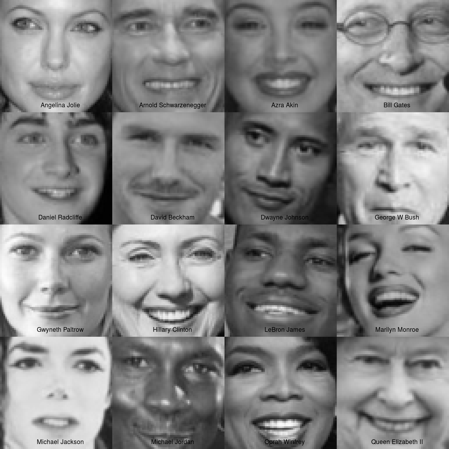
Figure 3.1: Each face in our dataset.
3.1 Prep for PCA
Collapse each image into one column of a matrix.
## collapse the grey matrix
face_data <- lapply(faces, function(x) c(x@grey))
## each column is a face
face_data <- do.call('cbind',face_data)
colnames(face_data) <- names(faces)
## have a look at the data matrix
head(face_data)
##      Angelina Jolie Arnold Schwarzenegger Azra Akin Bill Gates Daniel Radcliffe
## [1,]      0.3921569             0.4274510 0.3019608  0.8235294        0.2000000
## [2,]      0.3960784             0.4274510 0.2901961  0.8313725        0.2392157
## [3,]      0.4039216             0.4235294 0.2862745  0.8313725        0.2745098
## [4,]      0.4039216             0.4274510 0.2745098  0.8313725        0.3058824
## [5,]      0.4235294             0.4352941 0.2745098  0.8235294        0.3176471
## [6,]      0.4392157             0.4431373 0.2666667  0.8274510        0.3254902
##      David Beckham Dwayne Johnson George W Bush Gwyneth Paltrow Hillary Clinton
## [1,]     0.3058824      0.2235294     0.5529412       0.7411765       0.2705882
## [2,]     0.3333333      0.2313725     0.5607843       0.7843137       0.3176471
## [3,]     0.3921569      0.2274510     0.5490196       0.8117647       0.3686275
## [4,]     0.4470588      0.2078431     0.5686275       0.8313725       0.4745098
## [5,]     0.4862745      0.2039216     0.5803922       0.8313725       0.5686275
## [6,]     0.5254902      0.1960784     0.5450980       0.8352941       0.6470588
##      LeBron James Marilyn Monroe Michael Jackson Michael Jordan Oprah Winfrey
## [1,]    0.5333333     0.08627451       0.1529412      0.3372549     0.1372549
## [2,]    0.5254902     0.11764706       0.1647059      0.3411765     0.1607843
## [3,]    0.5333333     0.16470588       0.2078431      0.3411765     0.1686275
## [4,]    0.5215686     0.17647059       0.2549020      0.3450980     0.1764706
## [5,]    0.5294118     0.14117647       0.3176471      0.3411765     0.1647059
## [6,]    0.5490196     0.13333333       0.4039216      0.3137255     0.1960784
##      Queen Elizabeth II
## [1,]          0.1725490
## [2,]          0.1921569
## [3,]          0.2078431
## [4,]          0.2470588
## [5,]          0.2784314
## [6,]          0.3254902
3.1.1 Center around mean
## center around mean
mean <- apply(face_data, 1, mean)
mean_face <- pixmapGrey(mean, 64, 64, bbox = c(0, 0, 64, 64))
plot(mean_face)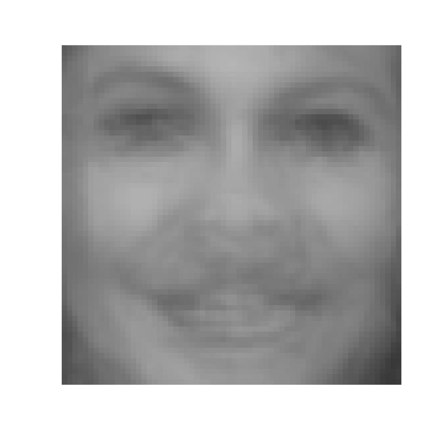
Figure 3.2: The 'mean' face from the 16 in our dataset.
centered <- apply(face_data, 2, function(x) x - mean)
## centered images
par(mfrow = c(4,4), mar = c(0,0,0,0), oma = c(0,0,0,0))
for(i in 1:length(faces)){
    plot(pixmapGrey(centered[,i], 64, 64, bbox = c(0, 0, 64, 64)))
    legend("bottom", bty = "n", paste(names(faces[i]), "centered", sep = " "))
}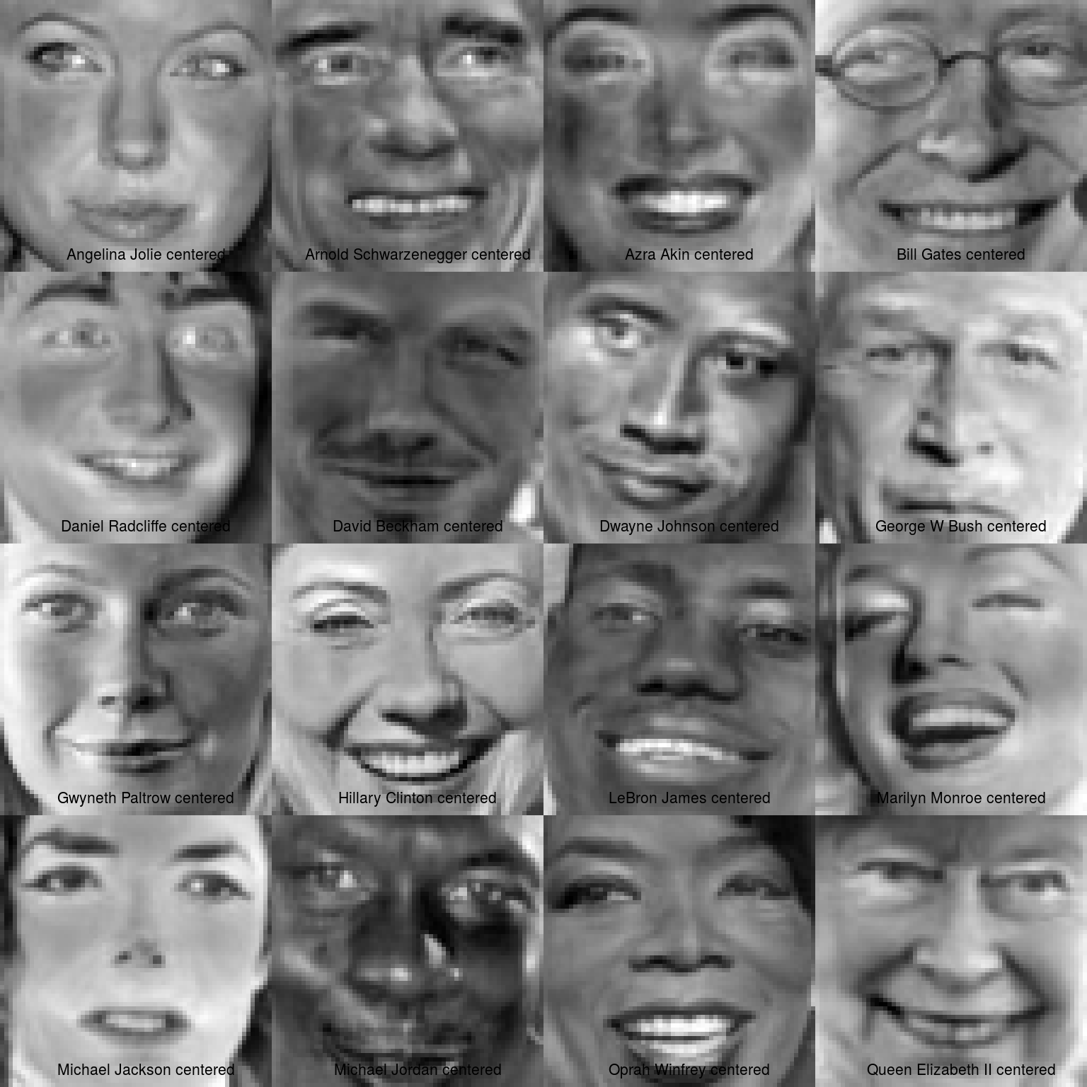
Figure 3.3: Each face centered (i.e., with the mean face subtracted).
3.2 Principal Component Analysis (PCA)
pca <- prcomp(centered)
summary(pca)
## Importance of components:
##                           PC1    PC2     PC3    PC4     PC5     PC6     PC7
## Standard deviation     0.2824 0.2135 0.15918 0.1511 0.13552 0.12660 0.11789
## Proportion of Variance 0.2811 0.1605 0.08928 0.0805 0.06471 0.05647 0.04897
## Cumulative Proportion  0.2811 0.4416 0.53088 0.6114 0.67609 0.73256 0.78153
##                            PC8     PC9    PC10    PC11    PC12    PC13    PC14
## Standard deviation     0.11556 0.10636 0.09315 0.09213 0.08201 0.07425 0.06766
## Proportion of Variance 0.04705 0.03986 0.03057 0.02990 0.02370 0.01943 0.01613
## Cumulative Proportion  0.82858 0.86843 0.89901 0.92891 0.95261 0.97204 0.98817
##                           PC15      PC16
## Standard deviation     0.05796 2.689e-16
## Proportion of Variance 0.01183 0.000e+00
## Cumulative Proportion  1.00000 1.000e+00
The PCA object, pca, contains the following information:
- the center point (
$center), - scaling (
$scale), and - standard deviation (
$sdev) of each principal component, as well as - the principal components (
$rotation), and - the values of each sample in terms of the principal components (
$x)
## for a nice biplot
library(ggfortify)
library(ggplot2)
## using autoplot
## PC1 vs PC2 by default
autoplot(pca,loadings = TRUE,loadings.label = TRUE,alpha = 0.1)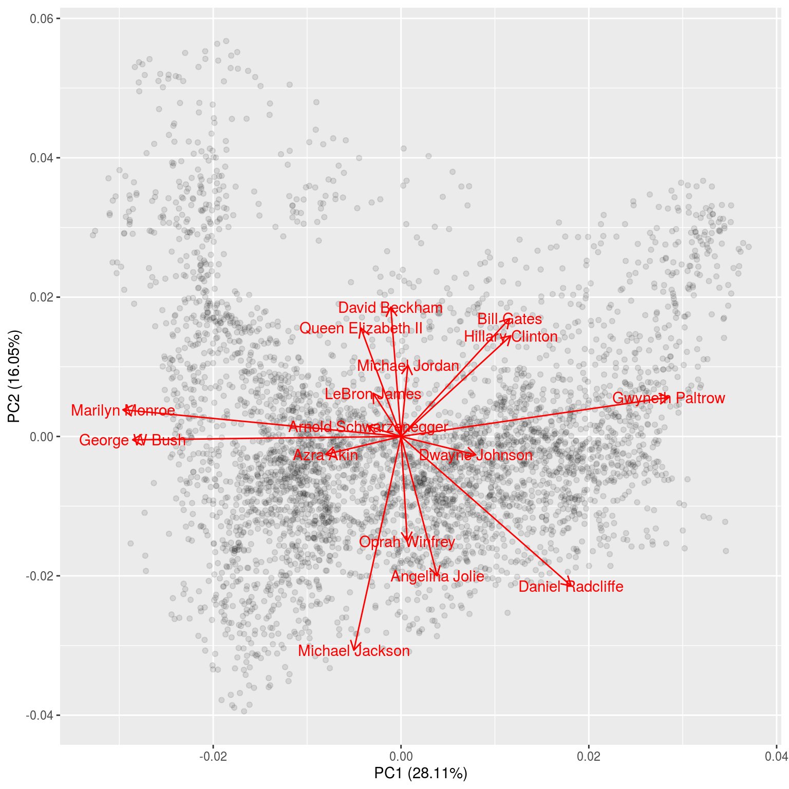
## play around with the arguments to see what they control
autoplot(pca,x = 3, y = 4,loadings = TRUE,loadings.label = TRUE,alpha = 0.1)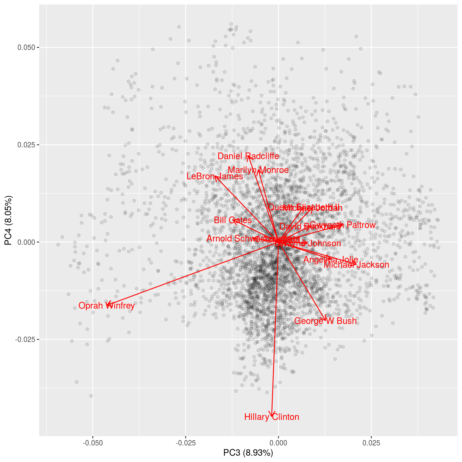
3.2.1 Eigenfaces (Principal Components)
## eigen faces
pcs <- pca$x
eigenfaces <- apply(pcs,2, function(x)  pixmapGrey(x, 64, 64, bbox = c(0, 0, 64, 64)))
par(mfrow = c(4,4), mar = c(0,0,0,0), oma = c(0,0,0,0))
for(i in 1:length(eigenfaces)){
    plot(eigenfaces[[i]])
    legend("bottom", bty = "n", paste("PC", i, sep = " "))
}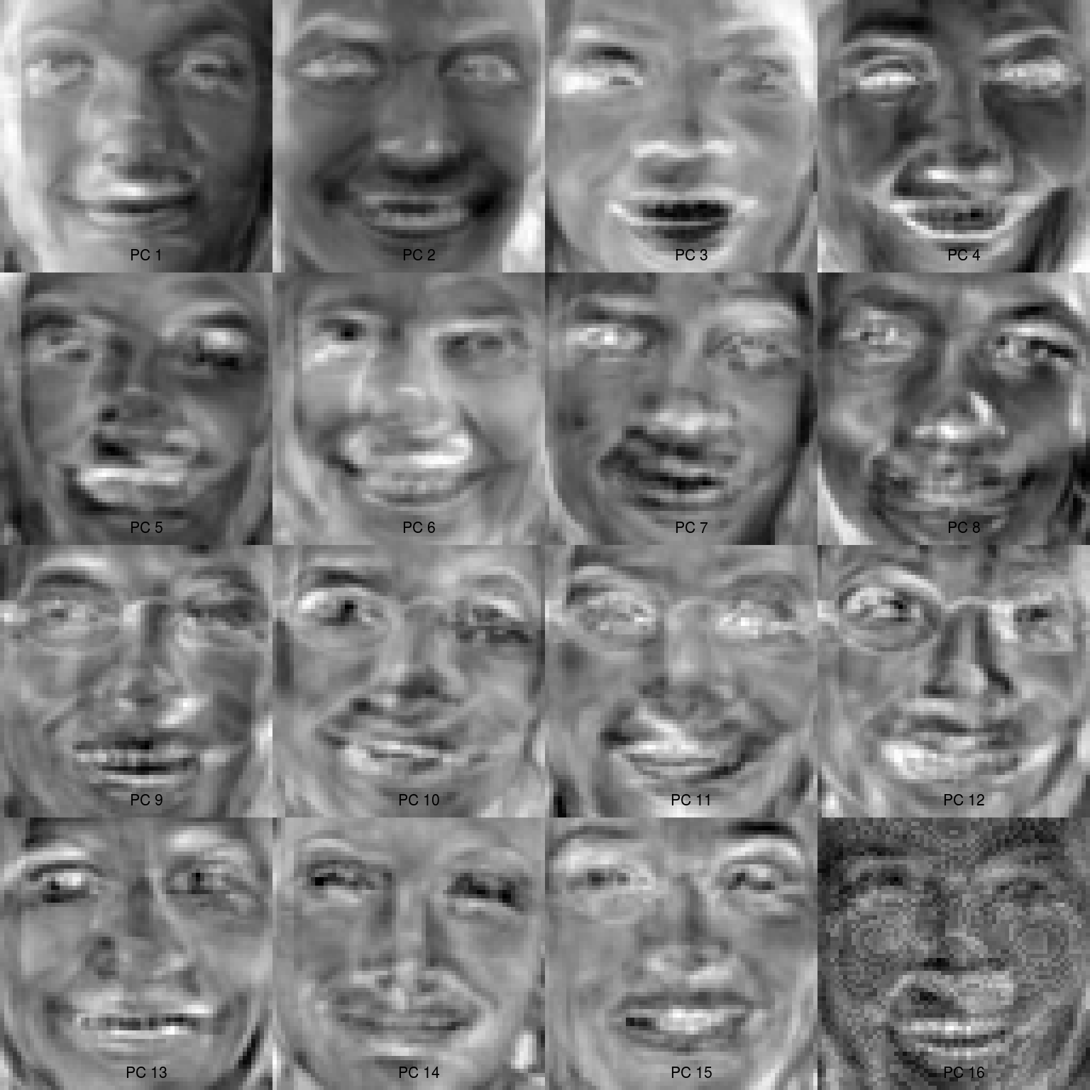
Figure 3.4: Each eigenface (PC1 to PC16). Note how noisy the faces get.
3.2.2 Reconstructing
3.2.2.1 How many coponents should we keep?
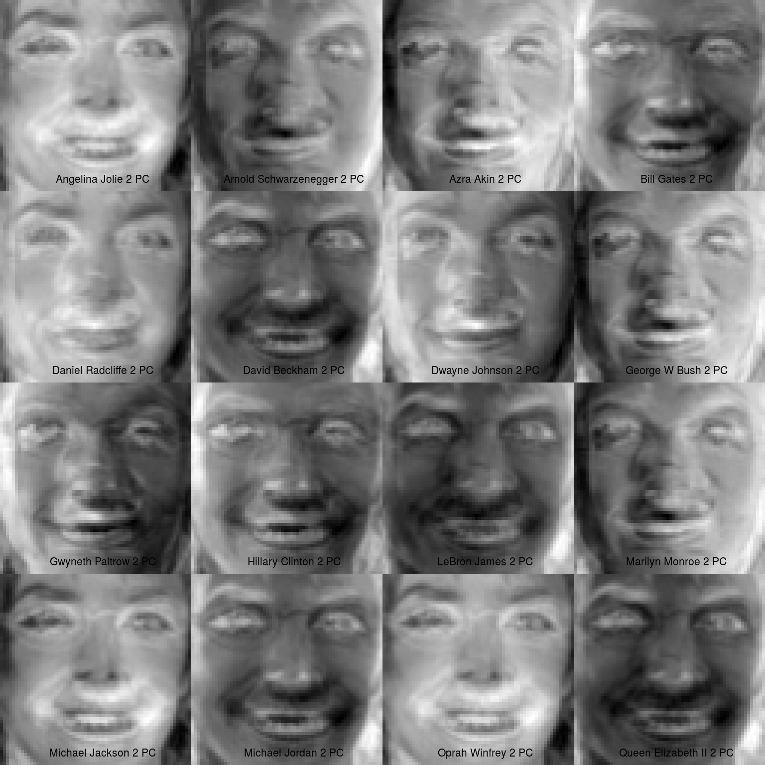
Each face is a weighted (loadings) combintation of the eigen faces (PCs) above, but how many PCs (eigenfaces) do we keep?
## screeplot
screeplot(pca,type = "lines", pch = 20)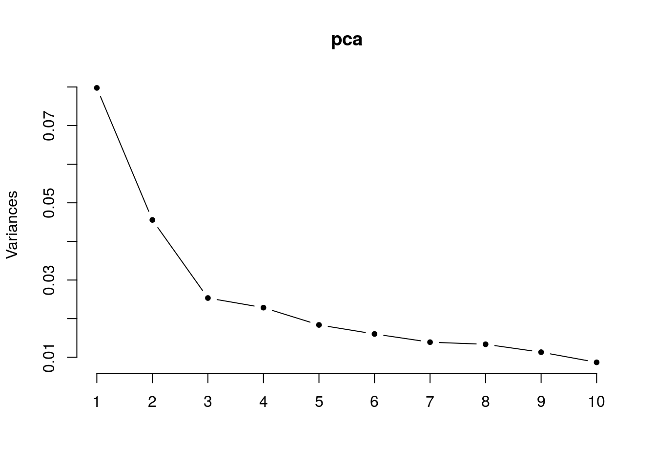
str(pca$rotation)
##  num [1:16, 1:16] 0.0668 -0.0609 -0.1394 0.2008 0.3148 ...
##  - attr(*, "dimnames")=List of 2
##   ..$ : chr [1:16] "Angelina Jolie" "Arnold Schwarzenegger" "Azra Akin" "Bill Gates" ...
##   ..$ : chr [1:16] "PC1" "PC2" "PC3" "PC4" ...
## 2 PCs
n_pc <- 2
recon <- pixm <- list()
for (i in 1:length(faces)){
recon[[i]] <- rowSums(pca$x[,1:n_pc]%*%pca$rotation[i,1:n_pc])
pixm[[i]] <- pixmapGrey(recon[[i]], 64, 64, bbox = c(0, 0, 64, 64))
}
## 2PC to reconstruct centered imags
par(mfrow = c(4,4), mar = c(0,0,0,0), oma = c(0,0,0,0))
for(i in 1:length(pixm)){
plot(pixm[[i]])
legend("bottom", bty = "n", paste(names(faces[i]), "2 PC", sep = " "))
}
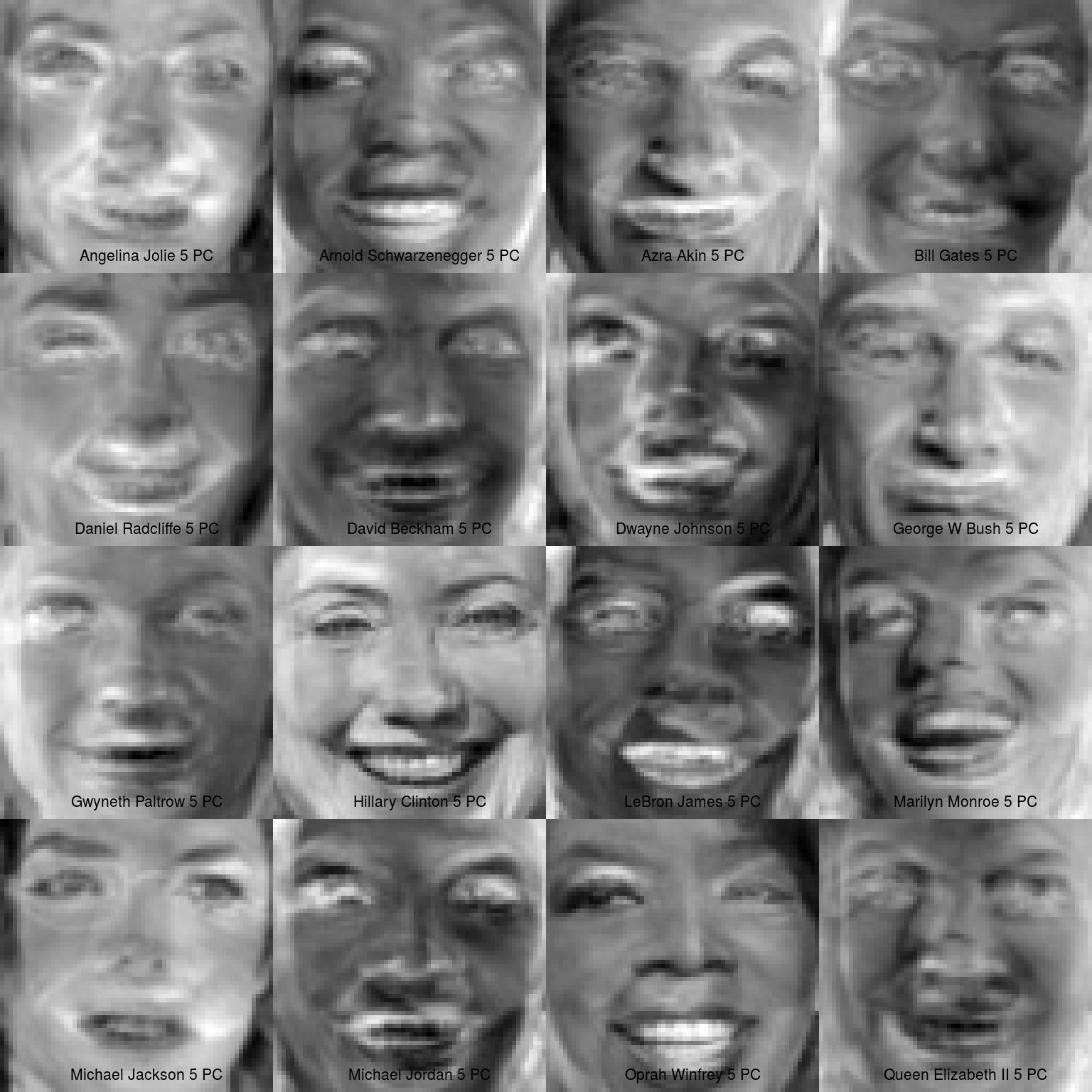
### Hmm OK, what about 5
## 5 PCs
n_pc <- 5

recon <- pixm <- list()
for (i in 1:length(faces)){
    recon[[i]] <- rowSums(pca$x[,1:n_pc]%*%pca$rotation[i,1:n_pc])
    pixm[[i]] <- pixmapGrey(recon[[i]], 64, 64, bbox = c(0, 0, 64, 64))
}

## 5PC to reconstruct centered images
par(mfrow = c(4,4), mar = c(0,0,0,0), oma = c(0,0,0,0))
for(i in 1:length(pixm)){
    plot(pixm[[i]])
    legend("bottom", bty = "n", paste(names(faces[i]), "5 PC", sep = " "))
}
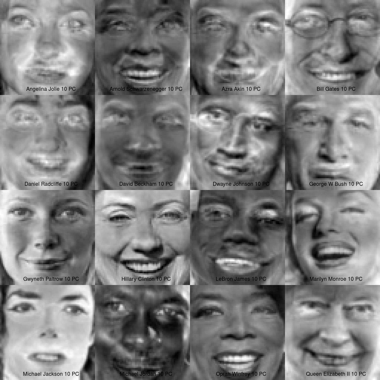
### Hmm OK, what about 10
## 10 PCs
n_pc <- 10

recon <- pixm <- list()
for (i in 1:length(faces)){
    recon[[i]] <- rowSums(pca$x[,1:n_pc]%*%pca$rotation[i,1:n_pc])
    pixm[[i]] <- pixmapGrey(recon[[i]], 64, 64, bbox = c(0, 0, 64, 64))
}
## 10PC to reconstruct centered images
par(mfrow = c(4,4), mar = c(0,0,0,0), oma = c(0,0,0,0))
for(i in 1:length(pixm)){
    plot(pixm[[i]])
    legend("bottom", bty = "n", paste(names(faces[i]), "10 PC", sep = " "))
}
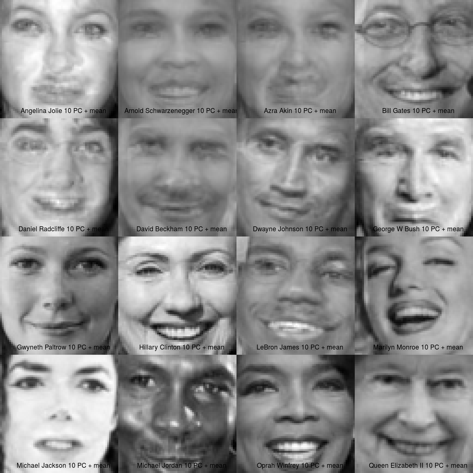
## remember this is the centered image, let's add the "mean face" to reconstruct the original
par(mfrow = c(4,4), mar = c(0,0,0,0), oma = c(0,0,0,0))
for(i in 1:length(recon)){
    plot(pixmapGrey(recon[[i]] + mean, 64, 64, bbox = c(0, 0, 64, 64)))
    legend("bottom", bty = "n", paste(names(faces[i]), "10 PC + mean", sep = " "))
}
3.3 1000 faces
Above we use only 16 images, but what if we had many, many, more. Then dimension reduction becomes much more useful. Here is a zipped archive of over 13,000 faces as grey pixmap images, as above.
We can download the archive, unzip, and read the files into R:
zip <- "http://conradsanderson.id.au/lfwcrop/lfwcrop_grey.zip"
temp <- tempfile(fileext = ".zip")
download.file(zip,destfile = temp)
tst <- unzip(temp)
unlink(temp)
all_faces <- list.files("lfwcrop_grey/faces",pattern = ".pgm", full = TRUE)
## read in a random subset of these images
## using set.seed to ensure the following is reproducible (means you will get the same subset)
set.seed(6666)
choose <- sample(1:length(all_faces), 1000, replace = FALSE)
face_set <- lapply(choose, function(x) read.pnm(all_faces[x]))
## name the object accordingly
col <- sapply(all_faces[choose], function(x) strsplit(strsplit(x,"faces/")[[1]][2],"_")[[1]])
names <-  sapply(col, function(y) paste(y[-length(y)],  collapse = " ")); names(names) <- NULL
head(names) ## if you've used the same seed as above this is what you should see
## [1] "Susilo Bambang Yudhoyono" "Brandon Larson"
## [3] "Kurt Warner"              "Toshihiko Fukui"
## [5] "Clemente de la Vega"      "Harvey Fierstein"
names(face_set) <- names
Mean face (of the 1000 faces)
## collapse the grey matrix
face_data <- lapply(face_set, function(x) c(x@grey))
## each column is a face
face_data <- do.call('cbind',face_data)
colnames(face_data) <- names(face_set)
## mean face
mean <- apply(face_data, 1, mean)
mean_face <- pixmapGrey(mean, 64, 64, bbox = c(0, 0, 64, 64))
plot(mean_face)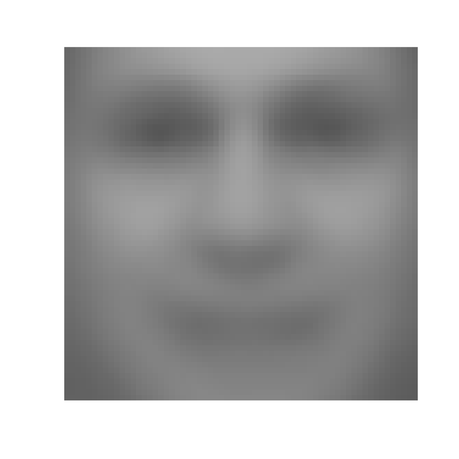
(#fig:collapse and meanface)The 'mean' face from the 1000 in our dataset. SPOOKY
PCA
centered <- apply(face_data, 2, function(x) x - mean)
pca <- prcomp(centered)
## screeplot
screeplot(pca,type = "lines", pch = 20)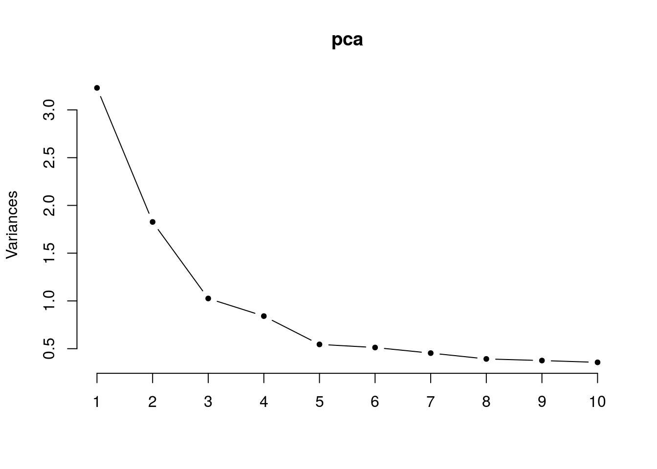
What does our first eigen face look like?
## eigen faces
pcs <- pca$x
eigenfaces <- apply(pcs,2, function(x)  pixmapGrey(x, 64, 64, bbox = c(0, 0, 64, 64)))
plot(eigenfaces[[1]])
legend("bottom", bty = "n", "PC 1")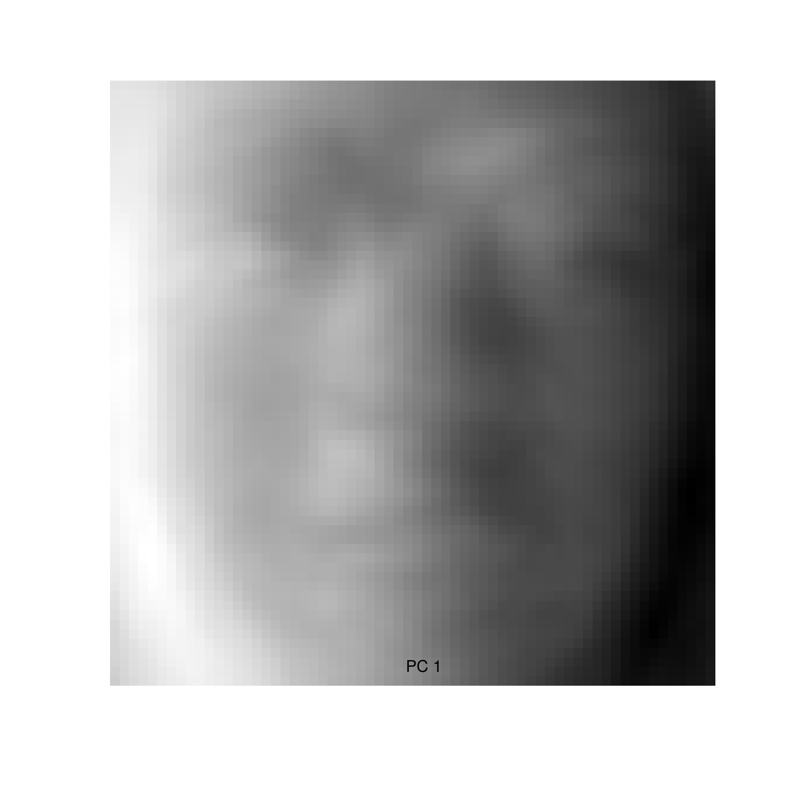
Figure 3.5: First eigenface (PC1).
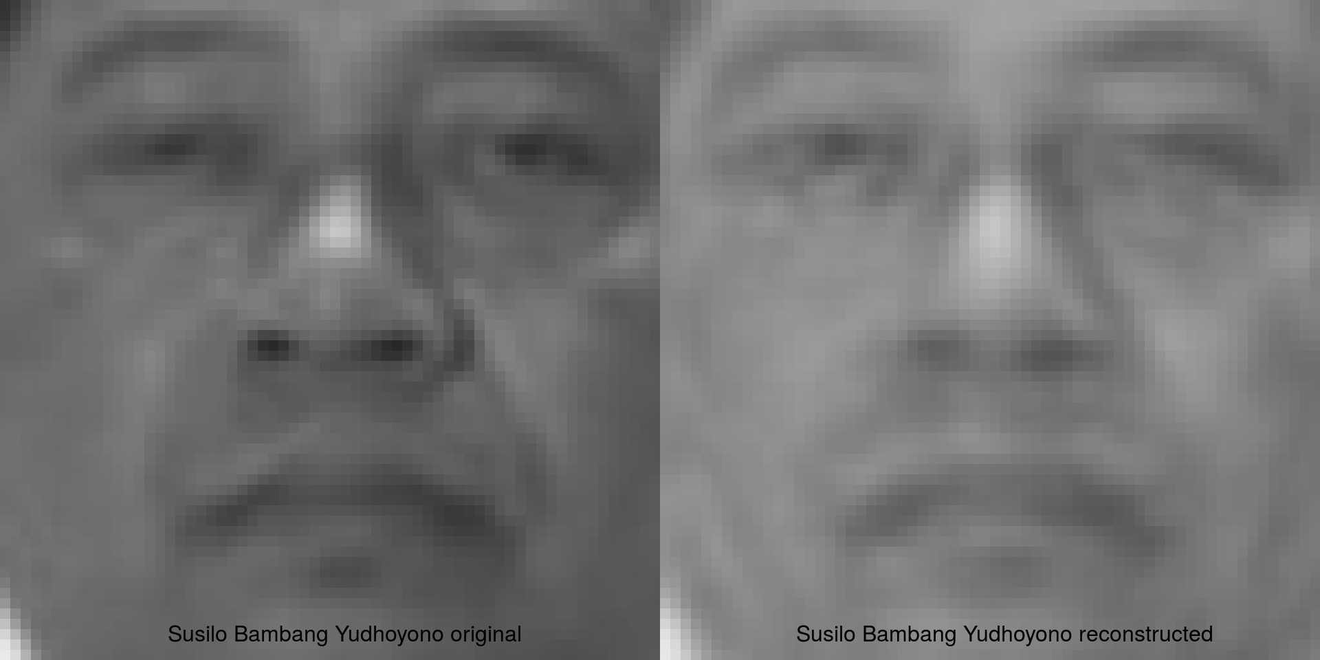
How many PCs would you keep? Let's try 200 (from a possible 1000) and recreate the first face in our dataset.
n_pc <- 200
recon <- rowSums(pca$x[,1:n_pc]%*%pca$rotation[1,1:n_pc])
## add the "mean face" to reconstruct the original
par(mfrow = c(1,2), mar = c(0,0,0,0), oma = c(0,0,0,0))
## original
plot(face_set[[1]])
legend("bottom", bty = "n", paste(names(face_set[1]), "original", sep = " "))
## reconstructed
plot(pixmapGrey(recon + mean, 64, 64, bbox = c(0, 0, 64, 64)))
legend("bottom", bty = "n", paste(names(face_set[1]), "reconstructed", sep = " "))